
PHYS 347: Optics
Instructor and Team Leader: Adam Green
This junior/senior level course focuses on physical optics: wave theory, polarization, interference, diffraction, and light-matter interactions. The first half of the course’s laboratory component deals with practical optical techniques, while the second half comprises a series of modern applications of those techniques. The laboratory is closely tied to lecture material, but missing from this course is a significant computational component, which would provide a more sophisticated link between theory and experiment. As a first step, we propose to develop additions to the two-part laboratory unit on polarized light, in which students will simulate and analyze optical systems using MATLAB. In the future, we will add similar modules to other portions of the class.
Laboratory #5: Creation and Manipulation of Polarized Light (Part 1: Imaging)
Conceptual goals: Understand the nature of polarized light, how polarization changes upon reflection and transmission, and how insects use polarized light for navigation and communication.
Computational goals: Use MATLAB’s Image Acquisition Toolbox to acquire images from CCD cameras. Learn basic image processing in MATLAB to create polarization maps of optical targets.
Experimental goal: Learn how to operate CCD cameras in conjunction with linear polarizers. Quantify how various materials either polarize or depolarize scattered light.
This first experiment in the polarized light lab introduces students to polarimetric imaging, a method that is widely used in science, engineering, and medicine. Using a CCD camera followed by a rotatable linear polarizer, they will acquire two images of an optical target with the Image Acquisition Toolbox. The first image is taken through the polarizer when its axis is horizontal, and the second image uses a vertical polarization axis. Students will process their images in MATLAB by taking the difference-over-sum of the two images to produce a map that quantifies how the target influences polarized light. Pixels on the map have values between zero and one, and they equal the scene’s “degree of polarization.” By applying an appropriate color palette to this map, students can optimize their visual sensitivity to small changes in polarization. Optical targets include dielectrics, metals, diffusers, commercial optical films, objects buried in turbid media, butterfly wings, and scarab beetle elytra. In this laboratory, special emphasis is placed on its application to insect vision. Many insects are very sensitive to polarized light and use it to identify mates as well as navigate during migration. The polarization maps that students create are meant to approximate what insects might see. The experimental portion of this project has already been developed and is largely based on our publication in the Physics Teacher [1]. (Eventually, this lab will incorporate a more complete version of imaging polarimetry, in which complete Stokes images are acquired. This work is in progress.)
Laboratory #5: Creation and Manipulation of Polarized Light (Part 2: Electro-optics)
Conceptual goals: Understand the nature of polarized light, how polarization changes upon reflection and transmission, and how it can be precisely manipulated and measured with modern instruments.
Computational goals: Learn how to use various linear algebra and plotting functions in MATLAB and MuPAD. Translate the matrix representation of polarized light into a simulation of an electro-optic modulator in order to understand experimental results and calibrate an optical system.
Experimental goal: Learn how to operate an electro-optic modulator and use it to control polarized light for a variety of polarimetry experiments.
In this second experiment with polarized light, students use two types of electro-optic modulators—liquid crystal retarders and photoelastic modulators—to precisely quantify the polarization properties of targets such as stretched plastic, compressed gelatin, sugar-water solutions, commercial polarizing elements, calcite crystals, and so on. We will develop a computational component for this laboratory in which students will translate the traditional matrix representations of polarized light into MATLAB simulations that can account for all possible combinations of static and time-varying polarizing elements, including targets of interest. Their programs will calculate output polarization states and plot irradiance curves for reflected and/or transmitted light. When students later perform their experiments, they will validate their program’s predictions by analyzing signals displayed on oscilloscopes and lock-in amplifiers. Results from simple, nearly ideal optical targets will initially build students’ confidence in both the physics and the simulations. Not only will the MATLAB simulations give students deeper understanding of polarized light, they will be essential for proper calibration of their optical systems. After calibration is complete, more complex optical targets will reveal the true power of the simulation because some materials affect polarized light in complicated ways that are tough to analyze with only paper and pencil. Much of the theoretical and experimental groundwork for this module is highlighted in our American Journal of Physics publication [2].
References:
1. A. S. Green, P. R. Ohmann, N. E. Leininger, and J. A. Kavanaugh, “Polarization Imaging and Insect Vision,” The Physics Teacher 48, 17 (January 2010).
2. K. J. Braun, C. R. Lytle, J. A. Kavanaugh, J. A. Thielen, and A. S. Green, “A Simple, Inexpensive Photoelastic Modulator,” American Journal of Physics 77 (1), 13 (2009).
Sample Results:
Here are some sample results of this project thus far. To test the suitability of the assignments for the Optics class and to develop them further, we presented our ideas to our student Elizabeth Annoni, who is a junior electrical engineering and physics double major. She did a fantastic job of writing codes for each assignment we gave her, and she invented and completed several other projects beyond what we originally proposed. Her excellent work serves as a foundation for further MATLAB development in Optics and other courses. We will continue to provide examples here as they become available.
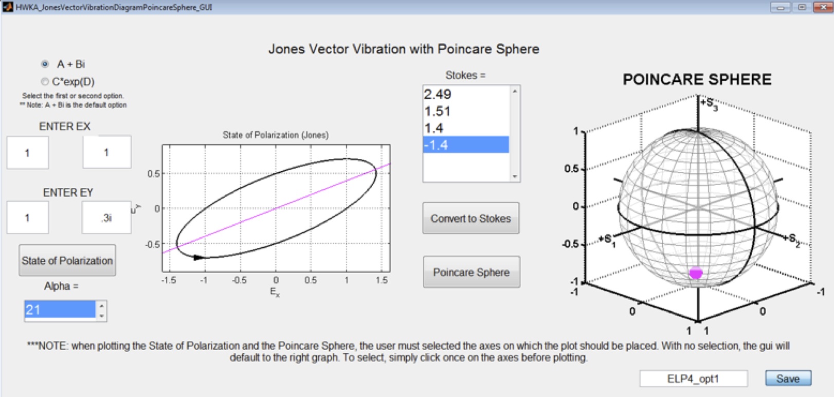
Example 1: Students first learn about the Jones and Stokes-Mueller matrix formalisms for polarized light. This GUI comprises modifications and a fusion of two programs available on the MathWorks file exchange page:
Light Polarization
Poincare Sphere Plot of Polarimetry Stokes Vectors
It allows students to enter a Jones vector, convert it to an un-normalized Stokes vector, and display the light’s corresponding vibration diagram as well as its representation on the (normalized) Poincare sphere.
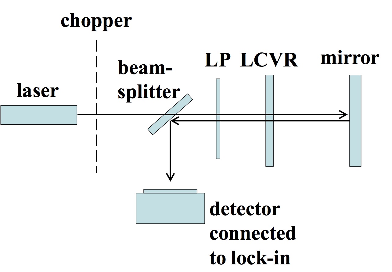
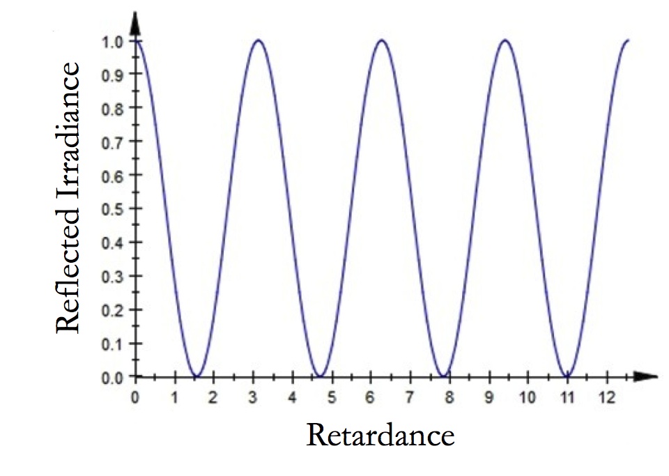
Example 2: Simulation of an optical isolation system that involves a liquid crystal variable retarder (LCVR). No light enters the detector if the linear polarizer (LP) and LCVR are oriented 45º apart and the LCVR is set to a multiple of quarter-wave retardance.
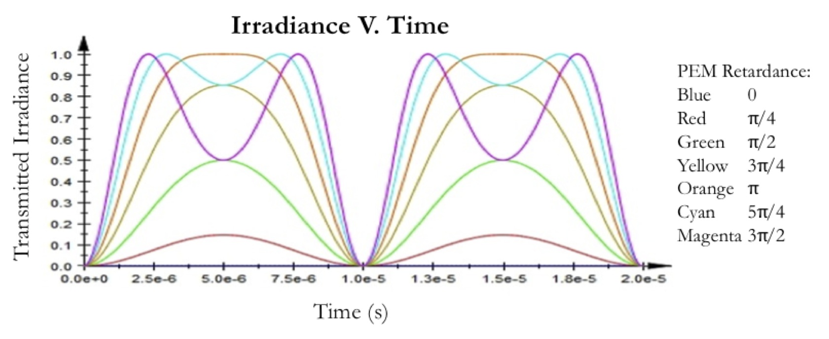
Example 3: Simulation of a photoelastic modulator placed between crossed linear polarizers. The maximum retardance is increased from 0 to 3 π / 2.
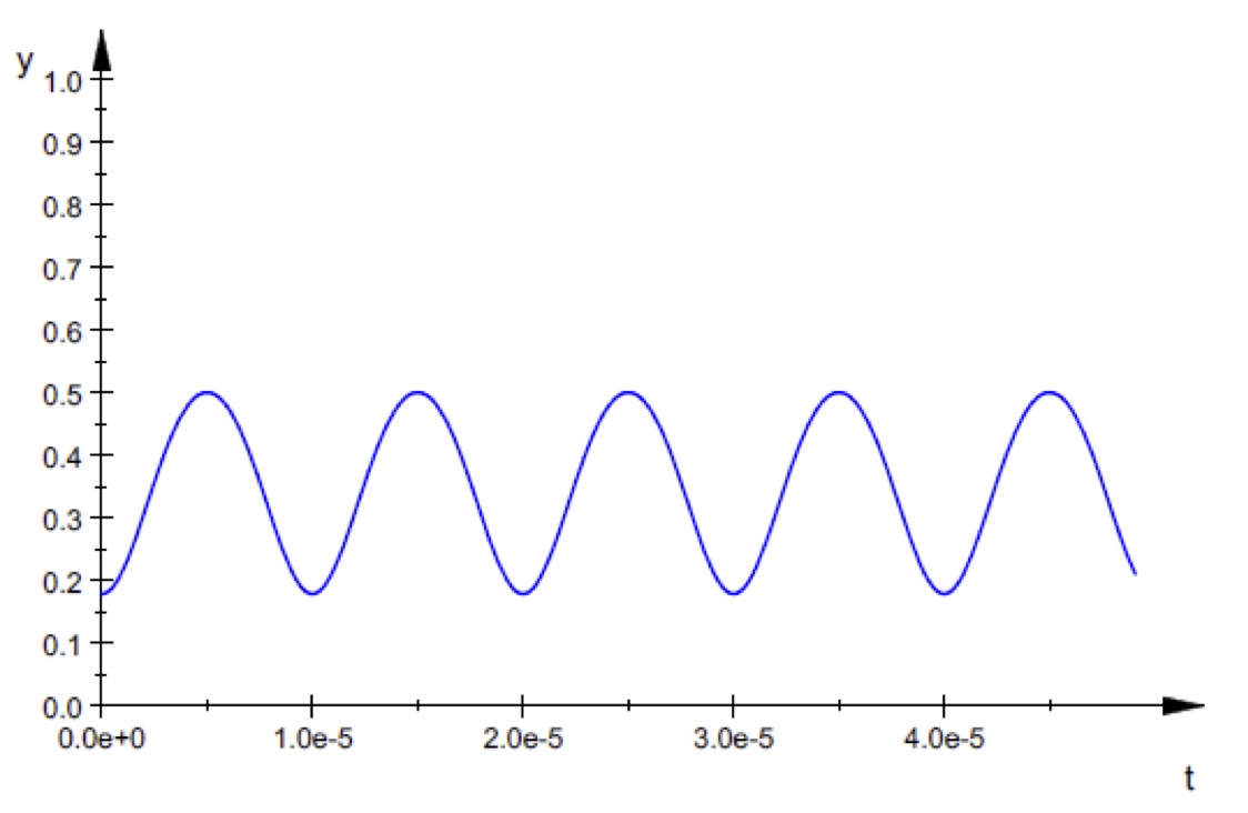
Example 4: Here is the irradiance output if the photoelastic modulator is set to quarter-wave maximum retardance and is followed by an optically active substance that rotates linearly polarized light through 25°.
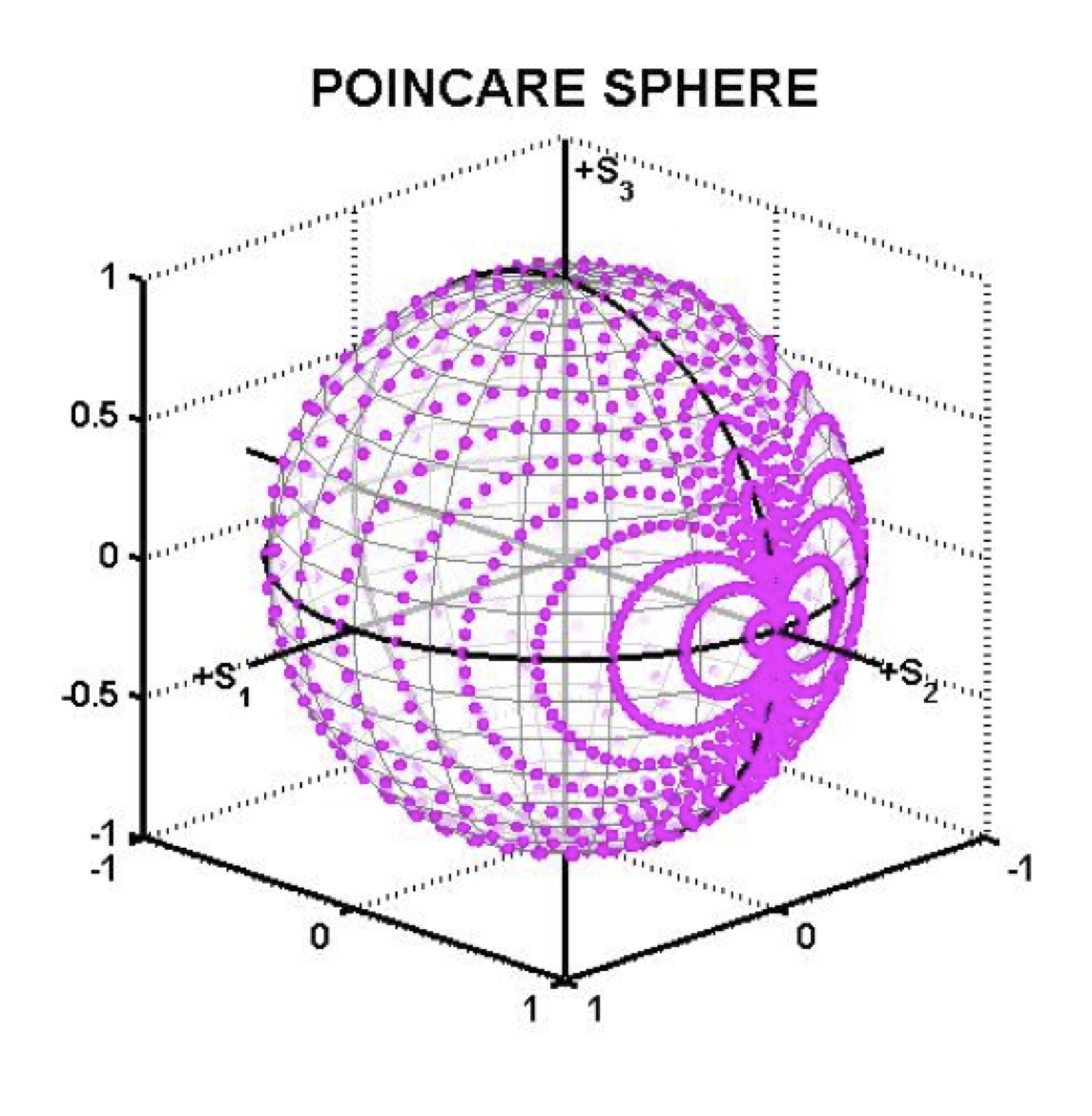
Example 5: Interpreting polarimetric systems using the Poincare sphere. This program is another modification of the one found on the previously mentioned MathWorks file exchange link. It allows students to customize the code and track the evolution of polarization states emerging from time-varying optical elements such as variable retarders, rotating polarizers and wave plates, etc. This example shows the output polarization states from a rotating, variable retarder when 45° linearly polarized light enters it. (The retarder’s phase shift varies from 0 to 2π, and its fast axis rotates through 2π.)
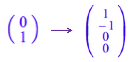
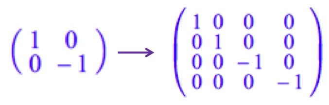
Example 6: Codes that convert from Jones vectors to Stokes vectors and from Jones matrices to Mueller matrices. (Note that the reverse conversions are not always possible because the Stokes-Mueller formalism can handle unpolarized light, but the Jones formalism cannot.)
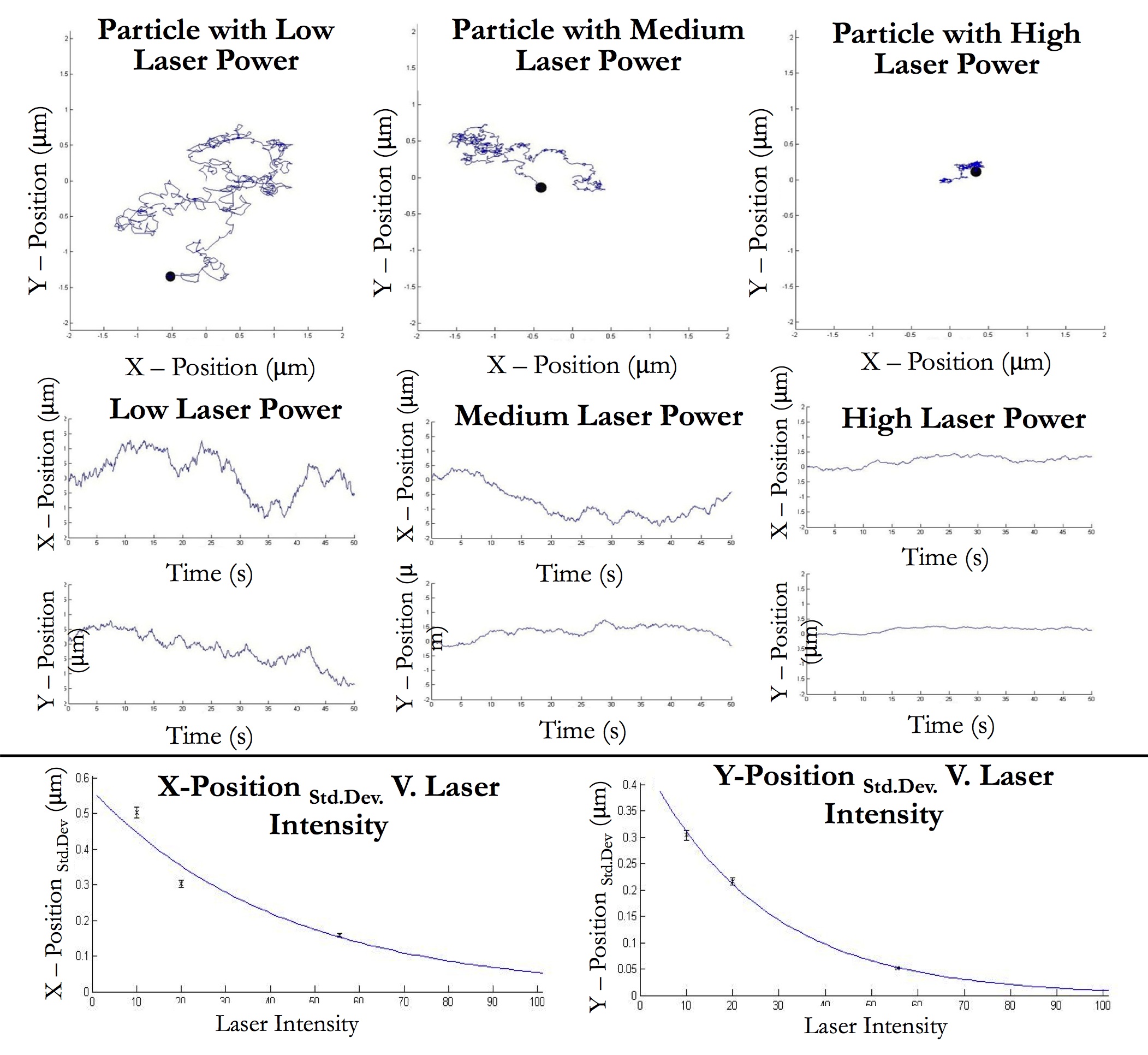
Example 7: (extension of original proposal) Rough simulation of Brownian motion of a microsphere trapped in an optical tweezers apparatus. The amplitude of motion decreases as trap strength increases. This program builds on one that students wrote the previous year in Modern Physics. Eventually, we will write a program that tracks and analyzes the motion of particles in videos acquired from our experimental apparatus.
Example 8: Polarization Imaging. [in progress]
This junior/senior level course focuses on physical optics: wave theory, polarization, interference, diffraction, and light-matter interactions. The first half of the course’s laboratory component deals with practical optical techniques, while the second half comprises a series of modern applications of those techniques. The laboratory is closely tied to lecture material, but missing from this course is a significant computational component, which would provide a more sophisticated link between theory and experiment. As a first step, we propose to develop additions to the two-part laboratory unit on polarized light, in which students will simulate and analyze optical systems using MATLAB. In the future, we will add similar modules to other portions of the class.
Laboratory #5: Creation and Manipulation of Polarized Light (Part 1: Imaging)
Conceptual goals: Understand the nature of polarized light, how polarization changes upon reflection and transmission, and how insects use polarized light for navigation and communication.
Computational goals: Use MATLAB’s Image Acquisition Toolbox to acquire images from CCD cameras. Learn basic image processing in MATLAB to create polarization maps of optical targets.
Experimental goal: Learn how to operate CCD cameras in conjunction with linear polarizers. Quantify how various materials either polarize or depolarize scattered light.
This first experiment in the polarized light lab introduces students to polarimetric imaging, a method that is widely used in science, engineering, and medicine. Using a CCD camera followed by a rotatable linear polarizer, they will acquire two images of an optical target with the Image Acquisition Toolbox. The first image is taken through the polarizer when its axis is horizontal, and the second image uses a vertical polarization axis. Students will process their images in MATLAB by taking the difference-over-sum of the two images to produce a map that quantifies how the target influences polarized light. Pixels on the map have values between zero and one, and they equal the scene’s “degree of polarization.” By applying an appropriate color palette to this map, students can optimize their visual sensitivity to small changes in polarization. Optical targets include dielectrics, metals, diffusers, commercial optical films, objects buried in turbid media, butterfly wings, and scarab beetle elytra. In this laboratory, special emphasis is placed on its application to insect vision. Many insects are very sensitive to polarized light and use it to identify mates as well as navigate during migration. The polarization maps that students create are meant to approximate what insects might see. The experimental portion of this project has already been developed and is largely based on our publication in the Physics Teacher [1]. (Eventually, this lab will incorporate a more complete version of imaging polarimetry, in which complete Stokes images are acquired. This work is in progress.)
Laboratory #5: Creation and Manipulation of Polarized Light (Part 2: Electro-optics)
Conceptual goals: Understand the nature of polarized light, how polarization changes upon reflection and transmission, and how it can be precisely manipulated and measured with modern instruments.
Computational goals: Learn how to use various linear algebra and plotting functions in MATLAB and MuPAD. Translate the matrix representation of polarized light into a simulation of an electro-optic modulator in order to understand experimental results and calibrate an optical system.
Experimental goal: Learn how to operate an electro-optic modulator and use it to control polarized light for a variety of polarimetry experiments.
In this second experiment with polarized light, students use two types of electro-optic modulators—liquid crystal retarders and photoelastic modulators—to precisely quantify the polarization properties of targets such as stretched plastic, compressed gelatin, sugar-water solutions, commercial polarizing elements, calcite crystals, and so on. We will develop a computational component for this laboratory in which students will translate the traditional matrix representations of polarized light into MATLAB simulations that can account for all possible combinations of static and time-varying polarizing elements, including targets of interest. Their programs will calculate output polarization states and plot irradiance curves for reflected and/or transmitted light. When students later perform their experiments, they will validate their program’s predictions by analyzing signals displayed on oscilloscopes and lock-in amplifiers. Results from simple, nearly ideal optical targets will initially build students’ confidence in both the physics and the simulations. Not only will the MATLAB simulations give students deeper understanding of polarized light, they will be essential for proper calibration of their optical systems. After calibration is complete, more complex optical targets will reveal the true power of the simulation because some materials affect polarized light in complicated ways that are tough to analyze with only paper and pencil. Much of the theoretical and experimental groundwork for this module is highlighted in our American Journal of Physics publication [2].
References:
1. A. S. Green, P. R. Ohmann, N. E. Leininger, and J. A. Kavanaugh, “Polarization Imaging and Insect Vision,” The Physics Teacher 48, 17 (January 2010).
2. K. J. Braun, C. R. Lytle, J. A. Kavanaugh, J. A. Thielen, and A. S. Green, “A Simple, Inexpensive Photoelastic Modulator,” American Journal of Physics 77 (1), 13 (2009).
Sample Results:
Here are some sample results of this project thus far. To test the suitability of the assignments for the Optics class and to develop them further, we presented our ideas to our student Elizabeth Annoni, who is a junior electrical engineering and physics double major. She did a fantastic job of writing codes for each assignment we gave her, and she invented and completed several other projects beyond what we originally proposed. Her excellent work serves as a foundation for further MATLAB development in Optics and other courses. We will continue to provide examples here as they become available.
Example 1: Students first learn about the Jones and Stokes-Mueller matrix formalisms for polarized light. This GUI comprises modifications and a fusion of two programs available on the MathWorks file exchange page:
Light Polarization
Poincare Sphere Plot of Polarimetry Stokes Vectors
It allows students to enter a Jones vector, convert it to an un-normalized Stokes vector, and display the light’s corresponding vibration diagram as well as its representation on the (normalized) Poincare sphere.
Example 2: Simulation of an optical isolation system that involves a liquid crystal variable retarder (LCVR). No light enters the detector if the linear polarizer (LP) and LCVR are oriented 45º apart and the LCVR is set to a multiple of quarter-wave retardance.
Example 3: Simulation of a photoelastic modulator placed between crossed linear polarizers. The maximum retardance is increased from 0 to 3 π / 2.
Example 4: Here is the irradiance output if the photoelastic modulator is set to quarter-wave maximum retardance and is followed by an optically active substance that rotates linearly polarized light through 25°.
Example 5: Interpreting polarimetric systems using the Poincare sphere. This program is another modification of the one found on the previously mentioned MathWorks file exchange link. It allows students to customize the code and track the evolution of polarization states emerging from time-varying optical elements such as variable retarders, rotating polarizers and wave plates, etc. This example shows the output polarization states from a rotating, variable retarder when 45° linearly polarized light enters it. (The retarder’s phase shift varies from 0 to 2π, and its fast axis rotates through 2π.)
Example 6: Codes that convert from Jones vectors to Stokes vectors and from Jones matrices to Mueller matrices. (Note that the reverse conversions are not always possible because the Stokes-Mueller formalism can handle unpolarized light, but the Jones formalism cannot.)
Example 7: (extension of original proposal) Rough simulation of Brownian motion of a microsphere trapped in an optical tweezers apparatus. The amplitude of motion decreases as trap strength increases. This program builds on one that students wrote the previous year in Modern Physics. Eventually, we will write a program that tracks and analyzes the motion of particles in videos acquired from our experimental apparatus.
Example 8: Polarization Imaging. [in progress]
If you are interested in using any of the materials found in this webpage in your own course, please contact us.