
PHYS 431: Quantum Mechanics
Instructor and Team Leader: Paul Ohmann
This one-semester course studies the fundamentals of quantum mechanics with mathematical rigor. Students are mostly seniors, though a few juniors typically take the class as well. Students in the class have all taken PHYS 225 Modern Physics, and most have taken PHYS 323 Methods of Experimental Physics, PHYS 331 Theoretical Mechanics, PHYS 341 Electricity and Magnetism, and PHYS 347 Optics. In that sense, PHYS 431 is a capstone course and can build on the knowledge and skills gained in the previous courses in our physics curriculum.
We previously incorporated a computational component as a final project in the course, developed through a previous NSF grant for computation. In this module, students calculate and plot several electron density functions for a hydrogen atom using the von Neumann accept/reject Monte-Carlo technique [1]. In our current effort, we have developed an additional computational project that builds explicitly on the two-week quantum dots lab that students perform in PHYS 225.
Homework Module: Modeling Quantum Dots as Infinite Spherical Wells
Conceptual goals: : Understand the connection between quantum dots and the infinite spherical well model.
Computational goals: Use MATLAB to numerically model the infinite spherical well for the l = 0 case that is appropriate for quantum dots. Compare the numerical results to the analytical solutions derived in class.
Experimental goal: Revisit the quantum dot system and understand how different wavelengths of light are produced from dots of different radii.
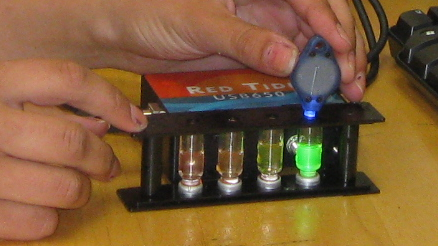
In PHYS 225, students spend one lab period measuring the spectral characteristics of several CdSe quantum dots, which are nano-scale semiconductors that can emit visible light, with frequencies that depend on the size of the dot. They then analyze and plot their results with MATLAB. In the subsequent lab period, students are introduced to the three-dimensional infinite square well as an initial model for the quantum dots, and they use MATLAB to numerically solve the corresponding Schrödinger equation using a finite-difference approximation. However, since quantum dots are roughly spherical, it would be far more appropriate to model them using the infinite spherical well. In PHYS 431, we analytically calculate the lowest order (l = 0) wavefunctions and corresponding energies for the infinite spherical well, and then discuss the higher order cases. Our class discussion leads naturally to this new computational exercise, in which students use MATLAB to numerically determine the solutions to the infinite spherical well for several values of l using Numerov’s method [2-3]. From our experience, we have found that students benefit from the additional exposure to numerical methods of solving differential equations (like the Schrödinger equation) in a system with which they are already familiar. Finally, our computational project asks students to relate their calculations to real quantum dot systems through a review of the literature.
References:
1. V. M. de Aquino, V. C. Aguilera-Navarro, M. Goto, and H. Iwamoto, “Monte-Carlo image representation,” Am. J. Phys. 69, 788-792 (2001).
2. Quiroz Gonzalez, J.L.M. and D. Thompson, “Getting started with Numerov’s method,” Computers in Physics 11(5), 514-5 (1997).
3. E. Hairer, S. P. Nørsett, and G. Wanner, Solving ordinary differential equations I: Nonstiff problems, Berlin, New York: Springer-Verlag (1993).
Sample Results:
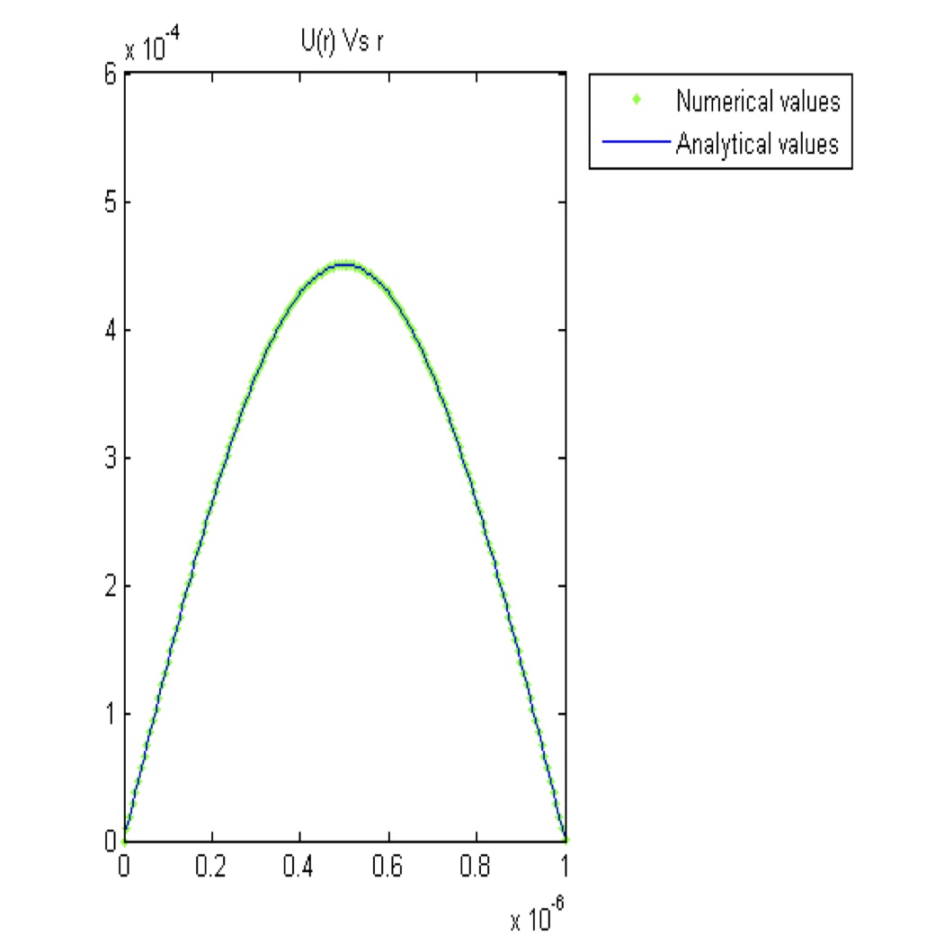
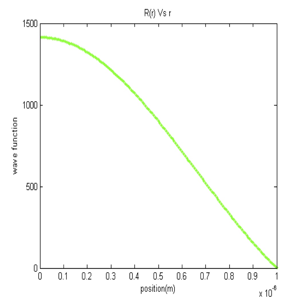
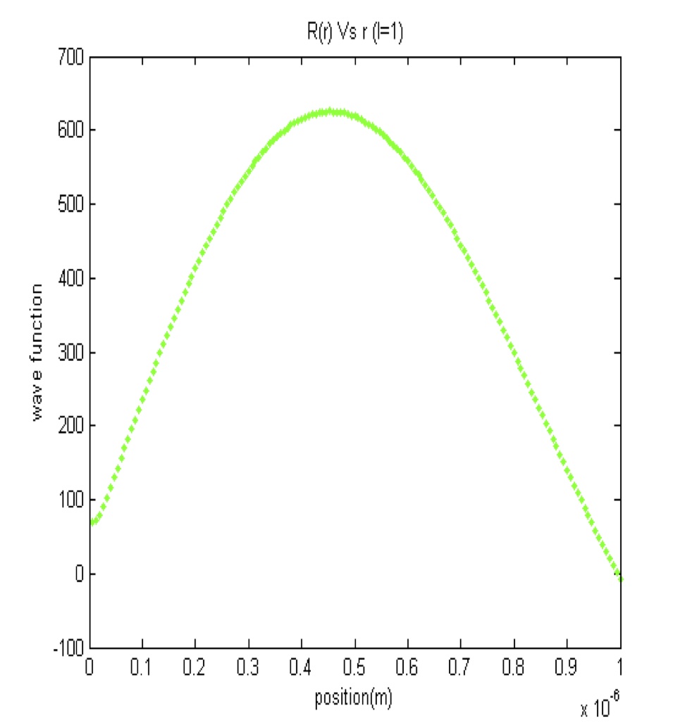
The plots below show the consistency between Numerov’s method and analytical solutions for the lowest order (l = 0) and next higher order (l = 1) wavefunctions. In each case the radial part of the wavefunction R(r) is plotted from the center of the quantum dot at r = 0 to its outer edge, which is taken rather arbitrarily to be 1.0 μm. An intermediate step is also shown, where we have substituted u(r) = r R(r) in order to simplify Schrödinger’s equation in spherical coordinates.
Fig. 1: u(r) vs. r (l=0) Fig. 2: R(r) vs. r (l=0)
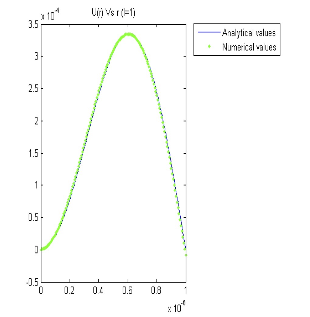
Fig. 3: U(r) vs r (l=1) Fig. 4: R(r) vs r (l=1)
For l > 0, the radial equation won’t be an ODE and so Numerov’s iteration becomes particularly important. Figures 3 and 4 show the l = 1 solution for u(r) and the radial wave function R(r).
This one-semester course studies the fundamentals of quantum mechanics with mathematical rigor. Students are mostly seniors, though a few juniors typically take the class as well. Students in the class have all taken PHYS 225 Modern Physics, and most have taken PHYS 323 Methods of Experimental Physics, PHYS 331 Theoretical Mechanics, PHYS 341 Electricity and Magnetism, and PHYS 347 Optics. In that sense, PHYS 431 is a capstone course and can build on the knowledge and skills gained in the previous courses in our physics curriculum.
We previously incorporated a computational component as a final project in the course, developed through a previous NSF grant for computation. In this module, students calculate and plot several electron density functions for a hydrogen atom using the von Neumann accept/reject Monte-Carlo technique [1]. In our current effort, we have developed an additional computational project that builds explicitly on the two-week quantum dots lab that students perform in PHYS 225.
Homework Module: Modeling Quantum Dots as Infinite Spherical Wells
Conceptual goals: : Understand the connection between quantum dots and the infinite spherical well model.
Computational goals: Use MATLAB to numerically model the infinite spherical well for the l = 0 case that is appropriate for quantum dots. Compare the numerical results to the analytical solutions derived in class.
Experimental goal: Revisit the quantum dot system and understand how different wavelengths of light are produced from dots of different radii.
In PHYS 225, students spend one lab period measuring the spectral characteristics of several CdSe quantum dots, which are nano-scale semiconductors that can emit visible light, with frequencies that depend on the size of the dot. They then analyze and plot their results with MATLAB. In the subsequent lab period, students are introduced to the three-dimensional infinite square well as an initial model for the quantum dots, and they use MATLAB to numerically solve the corresponding Schrödinger equation using a finite-difference approximation. However, since quantum dots are roughly spherical, it would be far more appropriate to model them using the infinite spherical well. In PHYS 431, we analytically calculate the lowest order (l = 0) wavefunctions and corresponding energies for the infinite spherical well, and then discuss the higher order cases. Our class discussion leads naturally to this new computational exercise, in which students use MATLAB to numerically determine the solutions to the infinite spherical well for several values of l using Numerov’s method [2-3]. From our experience, we have found that students benefit from the additional exposure to numerical methods of solving differential equations (like the Schrödinger equation) in a system with which they are already familiar. Finally, our computational project asks students to relate their calculations to real quantum dot systems through a review of the literature.
References:
1. V. M. de Aquino, V. C. Aguilera-Navarro, M. Goto, and H. Iwamoto, “Monte-Carlo image representation,” Am. J. Phys. 69, 788-792 (2001).
2. Quiroz Gonzalez, J.L.M. and D. Thompson, “Getting started with Numerov’s method,” Computers in Physics 11(5), 514-5 (1997).
3. E. Hairer, S. P. Nørsett, and G. Wanner, Solving ordinary differential equations I: Nonstiff problems, Berlin, New York: Springer-Verlag (1993).
Sample Results:
The plots below show the consistency between Numerov’s method and analytical solutions for the lowest order (l = 0) and next higher order (l = 1) wavefunctions. In each case the radial part of the wavefunction R(r) is plotted from the center of the quantum dot at r = 0 to its outer edge, which is taken rather arbitrarily to be 1.0 μm. An intermediate step is also shown, where we have substituted u(r) = r R(r) in order to simplify Schrödinger’s equation in spherical coordinates.
Fig. 1: u(r) vs. r (l=0) Fig. 2: R(r) vs. r (l=0)
Fig. 3: U(r) vs r (l=1) Fig. 4: R(r) vs r (l=1)
For l > 0, the radial equation won’t be an ODE and so Numerov’s iteration becomes particularly important. Figures 3 and 4 show the l = 1 solution for u(r) and the radial wave function R(r).
If you are interested in using any of the materials found in this webpage in your own course, please contact us.